Volumetrics with UAS Data
Introduction
Creating a New Feature Class
Using the Editor Tool to create polygons
Now you can use the editor tool to draw a polygon around the area of your choosing, double clicking to finish the polygon. Then go to the previously mentioned "Editor" drop-down menu, click "Stop Editing", and save the polygon.
Using the Extract by Mask tool
Next, using the search function, find the Extract by Mask tool and open it. There will be a window (shown in Figure 7) where you select the Input Raster (what you want to clip from), the "Input Raster or feature mask data" (the area you want to clip), and the Output Raster (the clipped version of the input).
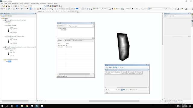
For Input Raster, select the raster that you want to clip from, in this case the DSM. The Input Raster or feature mask data will be the new feature class that was created previously. The Output raster should be placed in the .gbd folder that you are working in and named so that you can recognize what it is. The output should look something like Figure 8.
Looking that this clipped bit of DSM you can select the identify tool to click on the DSM to view the elevation at that specific location. Clicking on the outer edge of the polygon, where the DSM is darkest, you will be able to find a level that can be used as the base elevation as long as the area is not on a slope.
Using the Extracted Mask to calculate the volume
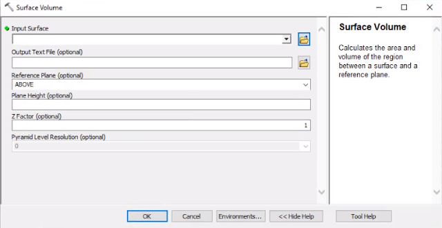
Use the search function to find the Surface Volume tool and open it up. Figure 9 shows the window.
Here the Input Surface will be the clipped DSM from the last step, the output text file should be placed where you will be able to find it and named so as to be recognizable, the reference plane will be "ABOVE" (since it is a pile and not a pit), and the plane height will be the elevation found using the identify tool. Clicking OK will begin processing the volume using the given parameters. The volume can be found in the table that will be displayed on the bottom of the table of contents pane. I have circled the location of the tables in Figure 10.
Resampling
Resampling allows you to compare the volumes of piles from multiple different flights/ data sets. Every flight, even if it is flown at the same altitude will have a different pixel cells resolution which is a problem when considering the calculations involved in acquiring pile volumes from a data set.
Resampling solves this problem by converting all the data sets to the same cell resolution.
To begin the resampling process use the tool search function and search resample. The resample tool window will look like Figure 11.
In this window the Input Raster will be the target of the resampling. It will be the file that has its cell resolution changed. The Output Raster Dataset will be what the Input Raster will be saved as once it has been resampled. The Output Cell Size is what cell resolution you want to match the Input Raster's cell resolution to (use this if you want don't want to set it manually). The X and Y will be the cell resolution that you set for the Input Raster, if you set the optional Output Cell Size this will be filled automatically.
Maps and Analysis For this resampling part of the lab I resampled clips of the same pile from three different dates so that I could compare their volumes and see how much the pile grew or shrank over time. Figure 12 is a map that I made to illustrate the changes in the pile over time.
This lab focuses on the calculations of volumes using UAS data. I use data retrieved from the wolfpaving data set that was seen in previous labs and go through the process of generating volumetric data in both Pix4D and ArcMap.
Methods
Pix4D Method
To start I opened Pix4D and the wolfpaving project file. The process here is explained in more detail in the "Processing Data in Pix4D with no GCPs" lab. Turn on the point cloud and turn off the cameras, rays, and tie points for easier viewing. On the left side of the window there is a cylinder shaped icon that will say "Volumes" as seen in Figure 1.
 |
| Figure 1: Volumes button |
From there, there will be a "New Volume" button in the volumes window (shown in Figure 2)
 |
| Figure 2: New Volume |
Clicking on that will allow you to click on the point cloud to draw a polygon around the base of whatever volume you are trying to calculate. Right clicking will finish the polygon and allow you to calculate the volume of whatever is above the polygon by clicking the calculate button in the volumes window. I repeated this process in the wolfpaving data set three times to calculate the volumes of three different piles as seen in Figure 3.
 |
| Figure 3: 3 Volumes |
This is quite an easy way of calculating the volumes of piles but it's accuracy is questionable since, in my experience, slightly different polygons could produce wildly different results.
ArcMap Method
Using ArcMap to calculate piles requires more steps to complete than Pix4D. This method uses both a hill shade and a DSM to isolate specified areas and calculate the volume above a user determined elevation. The hillshade will mostly be utilized by the user to be able to easily see and isolate the desired areas.
Creating a New Feature Class
To start, have ArcMap open with both a DSM and a hill shade of the wolfcreek data set. Then on the catalog pane on the left, right click on the .gbd file that the project is contained in, select "New", then click on "Feature Class..." as seen in Figure 4.
 |
| Figure 4: New Feature Class |
A new window will appear for creating the new feature class, bearing in mind that this will be a polygon meant to isolate a specified area, name it. Figure 5 shows the window that appears.
 |
| Figure 5: New Feature Class |
Continuing through the process of creating a New Feature Class, make sure that it uses the same coordinate system that the DSM and Hill shade are using.
The next two steps should be fine by default until you reach the fields step. For labeling purposes, enter two new fields; a "pile name" field and a "cubic meters" field using the text and short integer data types respectively.
Repeat this process for every separate volume area that you will be calculating.
Using the Editor Tool to create polygons
Now, to begin creating the polygons and demarcating the areas you will be working with, open the editor toolbar by clicking on the button shown below.
In the editor toolbar, clicking on the word "Editor" will open a drop-down menu where you can click on "Start Editing" to open up more options in the Editor toolbar (shown in Figure 6).
Then, on the far right of the toolbar, there will be a button called "Create Features" (looks like a pencil with a list), click on that button and, in the pane that opens up on the right you can select the new features that you created earlier.
Selecting one of them will allow you to choose what tools you want to use when constructing this feature at the bottom of the pane. For this purpose of this lab, I used the polygon tool but the other tools may be more useful depending on the shape of your desired area.
| Figure 6: Editor Toolbar |
Selecting one of them will allow you to choose what tools you want to use when constructing this feature at the bottom of the pane. For this purpose of this lab, I used the polygon tool but the other tools may be more useful depending on the shape of your desired area.
Now you can use the editor tool to draw a polygon around the area of your choosing, double clicking to finish the polygon. Then go to the previously mentioned "Editor" drop-down menu, click "Stop Editing", and save the polygon.
Repeat this process for every separate volume area that you will be calculating.
Using the Extract by Mask tool
Next, using the search function, find the Extract by Mask tool and open it. There will be a window (shown in Figure 7) where you select the Input Raster (what you want to clip from), the "Input Raster or feature mask data" (the area you want to clip), and the Output Raster (the clipped version of the input).
 |
| Figure 7: Extract by Mask window |
 |
| Figure 8: Pile A Clipped |
Using the Extracted Mask to calculate the volume
Use the search function to find the Surface Volume tool and open it up. Figure 9 shows the window.
 |
| Figure 9: Surface Volume Window |
 |
| Figure 10: Data Tables |
Repeat this process for each pile.
Resampling allows you to compare the volumes of piles from multiple different flights/ data sets. Every flight, even if it is flown at the same altitude will have a different pixel cells resolution which is a problem when considering the calculations involved in acquiring pile volumes from a data set.
Resampling solves this problem by converting all the data sets to the same cell resolution.
To begin the resampling process use the tool search function and search resample. The resample tool window will look like Figure 11.
 |
| Figure 11: Resampling Window |
Maps and Analysis For this resampling part of the lab I resampled clips of the same pile from three different dates so that I could compare their volumes and see how much the pile grew or shrank over time. Figure 12 is a map that I made to illustrate the changes in the pile over time.
 |
| Figure 12: Litchfield Pile Volumes |
And here is a table for the Litchfield Pile Volumes:
Date
|
Volume
|
July 22
|
98563.998493
|
August 27
|
142150.80792
|
September 30
|
101508.984285
|
And this is just because I like charts (Figure 13):
 |
| Figure 13: A line chart? |
As you can see, the pile returned to just about its original volume after growing in August event though it is shaped completely different.
Wolf Creek Map and Comparison to Pix4D
Here is the map that I made for the first part of the lab. (Figure 14)
 |
| Figure 14: Wolf Creek Pile Volumes Map |
I don't feel the need to make a chart for this map since I'm not really comparing them. This part of the lab was more of a proof of concept, that this method could be used to find the volumes of the piles.
In comparing the results from ArcMap and Pix4D, however, there were quite significant differences.
ArcMap
|
Pix4D
|
Percent Difference
| |
Pile A
|
713.734
|
442.64
|
46.9%
|
Pile B
|
2565.59
|
2126.31
|
18.7%
|
Pile C
|
14686.766
|
10906.33
|
29.5%
|
Figure 15 is a bar chart comparing the differences between the calculated volumes in Pix4D and ArcMap.
 |
| Figure 15: Volume Collection Comparisons |
While I acknowledge that I am, by no means, an expert in collecting the volume of piles, it is my belief that there is a certain unacceptable of inaccuracy in one of these methods (I'm assuming Pix4D since it's not a GIS software) if a high level of accuracy is necessary.
Conclusion
UAS valuable in volumetrics because is both easier and more reliable than other methods of measuring volume of a given pile or pit (perhaps a body of water if the right sensors are used?) Where previously, you had to use approximations using geometric formulas to find volumes, now you can use UAS and computer software to find much more exact data. While this is still not a perfect method, the technology is improving all the time and is already better than the alternative which relies on estimations and set formulas for known 3D shapes.
.

